Staircase basics

Stairs is a class in the staircase package. It is a data structure, with associated methods, for modelling and manipulating step functions. We will often use the terms step function and Stairs instance interchangeably. A step function is piecewise constant, that is it is composed of a sequence of intervals. Every interval has a start, an end, and a value. Most importantly though it is assumed that there are no gaps between intervals in the sequence. When a Stairs instance is created it already holds one interval - this interval extends from -infinity to +infinity and its value can be specified at creation. A Stairs instance will always hold start and end with an interval of infinite length (and these may be the same interval).

import matplotlib.pyplot as plt
import pandas as pd
import numpy as np
import staircase as sc

Let’s create two Stairs instances to play with. By default they will have one interval (-inf, inf) with a value of 0. We can check that they are the equivalent too.

s1 = sc.Stairs()
s2 = sc.Stairs()
assert s1 == s2
assert not s1 != s2

/home/docs/checkouts/readthedocs.org/user_builds/railing/envs/v1.6.4/lib/python3.8/site-packages/ipykernel/ipkernel.py:283: DeprecationWarning: `should_run_async` will not call `transform_cell` automatically in the future. Please pass the result to `transformed_cell` argument and any exception that happen during thetransform in `preprocessing_exc_tuple` in IPython 7.17 and above.
  and should_run_async(code)

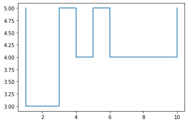
Let’s now add two intervals to s1. Each Stairs instance has a function “layer” which can be used to layer intervals to the existing ones. The parameters to the function are ‘start’, ‘end’ and ‘value’ respectively.

s1.layer(1,3,2)
s1.layer(6,10,1)

<staircase.Stairs, id=139759805251840, dates=False>

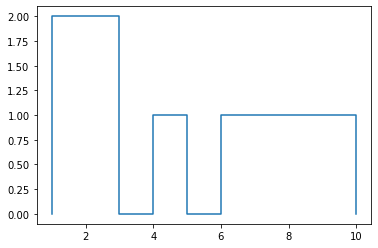
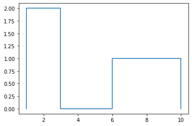
The Stairs class has a plot function. By default it will not plot the two infinite intervals which begin and end the step function. Is the plot below what you expect it to be?

s1.plot()

<AxesSubplot:>

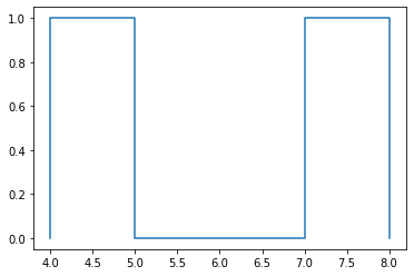
Let’s not leave s2 out of the fun. We’ll add a couple of intervals and plot.

s2.layer(4,5,1)
s2.layer(7,8,1)
s2.plot()

<AxesSubplot:>

The plot function can take an axes (from matplotlib) as an argument. It will plot to this axes, allowing us to put plots for multiple Stairs instances on the one chart.

fig, ax = plt.subplots()
s1.plot(ax)
s2.plot(ax)
plt.show()

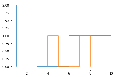
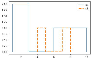
Some of the details are getting lost in the above chart. The plot function can also take a dictionary of keyword arguments that are typically used with matplotlib’s Line2D:

fig, ax = plt.subplots()
s1.plot(ax, label="s1")
s2.plot(ax, label = "s2", linestyle="--", linewidth=3)
ax.legend()
plt.show()

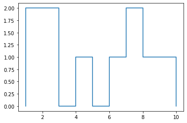
As much fun as plotting step functions is, the main purpose of the Stairs class is to provide an arithmetic with these structures, so that we can add, subtract, take minimums, maximums and means etc. Below the maximum is calculated between s1 and s2 and is plotted. Is the plot what you expect?

max_s1_s2 = sc.max([s1, s2])
max_s1_s2.plot()

<AxesSubplot:>

We can add Stairs instances

(s1 + s2).plot()

/home/docs/checkouts/readthedocs.org/user_builds/railing/envs/v1.6.4/lib/python3.8/site-packages/ipykernel/ipkernel.py:283: DeprecationWarning: `should_run_async` will not call `transform_cell` automatically in the future. Please pass the result to `transformed_cell` argument and any exception that happen during thetransform in `preprocessing_exc_tuple` in IPython 7.17 and above.
  and should_run_async(code)

<AxesSubplot:>

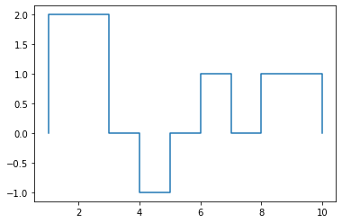
We can subtract Stairs instances

(s1 - s2).plot()

<AxesSubplot:>

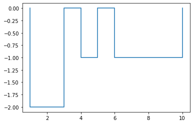
We can invert Stairs instances

(-max_s1_s2).plot()

<AxesSubplot:>

In the below example we initialise a Stairs instance to extend from -inf to +inf with a value of 5, from which we subtract our max_is Stairs instance.

(sc.Stairs(5) - max_s1_s2).plot()

<AxesSubplot:>

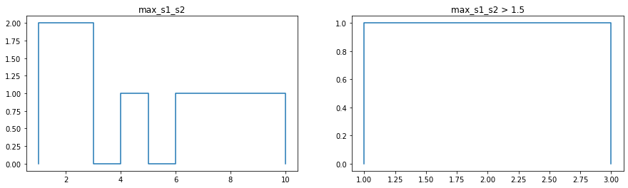
In the next example we want to see where our max_is Stairs instance is greater than 1.5 in value. Note that whenever we do comparisons, the result will always be a sequence of binary-valued intervals.

fig = plt.figure(figsize=(15, 4))

ax = fig.add_subplot(1,2,1)
ax.set_title("max_s1_s2")
max_s1_s2.plot(ax)

ax = fig.add_subplot(1,2,2)
ax.set_title("max_s1_s2 > 1.5")
(max_s1_s2 > 1.5).plot(ax)

<AxesSubplot:title={'center':'max_s1_s2 > 1.5'}>

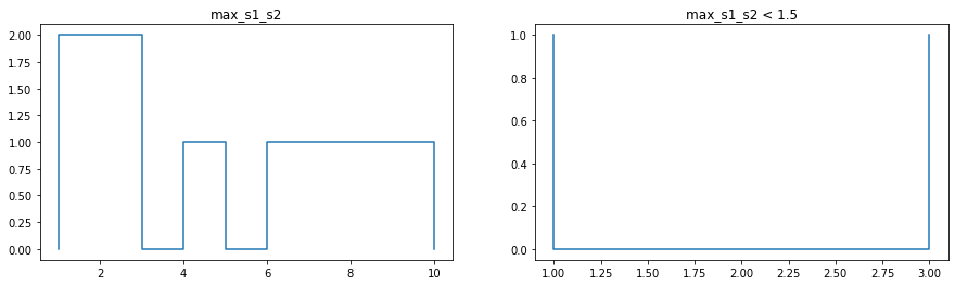
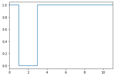
The below example is similar to the above but we are using less than, rather than greater than. You should expect that the result is the binary (i.e. boolean) opposite of the above result. Remember that infinite-length intervals are not plotted, so in the chart on the right, there are intervals (-inf, 1) and (3, inf) which have a value of 1.

fig = plt.figure(figsize=(15, 4))

ax = fig.add_subplot(1,2,1)
ax.set_title("max_s1_s2")
max_s1_s2.plot(ax)

ax = fig.add_subplot(1,2,2)
ax.set_title("max_s1_s2 < 1.5")
(max_s1_s2 < 1.5).plot(ax)

<AxesSubplot:title={'center':'max_s1_s2 < 1.5'}>

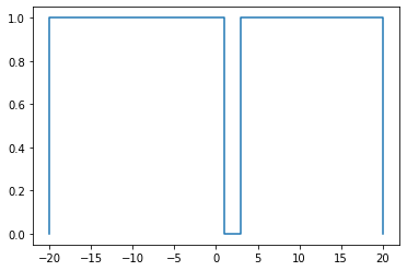
Although the above-right chart is correct, it can be easy to forget that about the infinite-length start and end intervals in the sequence. We can call the clip function, which sets the value of the Stairs instance, outside the range specified in the parameters to zero. This can make the resulting plot a little more easier to understand.

(max_s1_s2 < 1.5).clip(-20,20).plot()

<AxesSubplot:>

Additionally, we can combine the above approach with setting the x-axis limits, to get an even nicer solution

fig, ax = plt.subplots()
(max_s1_s2 < 1.5).clip(-100,100).plot(ax)
ax.set_xlim(0,11)
plt.show()

The Stairs class also has a function for finding the area under the graph: integrate(). Note that it does not calculate absolute values, so a step function consisting of negative values will result in a negative area. Negative areas and positive areas can cancel each other out. Check that you agree with the calculation below?

s1.plot()
print(f'The area under s1 is {s1.integrate()}')

The area under s1 is 8

**We can also restrict the range in which the IntervalSequence is integrated. Check that you agree with the calculation below, where we restrict the calculation to be between 2.5 and 3.

s1.integrate(2.5,3)

1.0

We can also use the mean function to calculate the average value. If the Stairs instance represents the utilisation of some thing over time, then the mean function can be used to calculate the average utilisation.

s1.mean()

0.8888888888888888

It is important to note that by default infinite-length intervals will not be included in the calculation. In the above example, the non-infinite length intervals occur in the range (1,10), so the mean will be calculated over this range by default. If we wanted to force the calculation over a particular range, eg. (0,10) then we can do this by supplying parameters to the mean function.

s1.mean(0,10)

0.8

If you would like to see the intervals of a Stairs instance expressed in a DataFrame then this is available

s1.plot()
s1.to_dataframe()

	start	end	value
0	-inf	1.0	0
1	1.0	3.0	2
2	3.0	6.0	0
3	6.0	10.0	1
4	10.0	inf	0

Under the hood the Stairs class is built upon a Sorted Dictionary - a dictionary where the keys, are always ordered in ascending order. The initial key should always be -inf and the corresponding value should be the value of the first interval (which always begins at -inf). The rest of the keys in the Sorted Dictionary represent the start/end points of the intervals and the values represent the change at that point. Does the following make sense?

s1

/home/docs/checkouts/readthedocs.org/user_builds/railing/envs/v1.6.4/lib/python3.8/site-packages/ipykernel/ipkernel.py:283: DeprecationWarning: `should_run_async` will not call `transform_cell` automatically in the future. Please pass the result to `transformed_cell` argument and any exception that happen during thetransform in `preprocessing_exc_tuple` in IPython 7.17 and above.
  and should_run_async(code)

<staircase.Stairs, id=139759805251840, dates=False>

Returning to equality comparisons, let’s look at what is returned in the below example where we compare two calculations which should be equal:

sc.Stairs(2) - s1 == -s1 + sc.Stairs(2)

<staircase.Stairs, id=139759764787104, dates=False>

The result was itself a Stairs instance, which contains just one interval: (-inf, inf) with a value of 1. This Stairs instance is special in that it evaluates to True when interpreted as a bool:

bool(sc.Stairs(2) - s1 == -s1 + sc.Stairs(2))

True

This is why we can use these comparisons as conditions:

if sc.Stairs(2) - s1 == -s1 + sc.Stairs(2):
    print("They are the same")
else:
    print("They are not the same")

They are the same

There is a function belonging to the Stairs class called make_boolean. Calling this function returns a Stairs instance where the values of the intervals are 0 if and only if the values of the original intervals were zero. This approach is consistent with the approach used for floats:

print(bool(0.3))
print(bool(1.3))
print(bool(-1))
print(bool(-0.3))
print(bool(0))

True
True
True
True
False

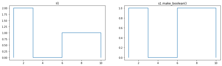
make_boolean() may not have many explicit uses but is used internally frequently. The following example illustrates its effect.

fig = plt.figure(figsize=(15, 4))

ax = fig.add_subplot(1,2,1)
ax.set_title("s1")
s1.plot(ax)

ax = fig.add_subplot(1,2,2)
ax.set_title("s1.make_boolean()")
s1.make_boolean().plot(ax)

<AxesSubplot:title={'center':'s1.make_boolean()'}>

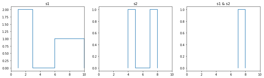
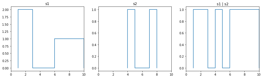
The implementation of ‘logical and’ and ‘logical or’ (& and | respectively) are some of the mechanisms which leverage the make_boolean function

fig = plt.figure(figsize=(15, 4))

ax = fig.add_subplot(1,3,1)
ax.set_title("s1")
ax.set_xlim(0,10)
s1.plot(ax)

ax = fig.add_subplot(1,3,2)
ax.set_title("s2")
ax.set_xlim(0,10)
s2.plot(ax)

ax = fig.add_subplot(1,3,3)
ax.set_title("s1 & s2")
ax.set_xlim(0,10)
(s1 & s2).plot(ax)

<AxesSubplot:title={'center':'s1 & s2'}>

fig = plt.figure(figsize=(15, 4))

ax = fig.add_subplot(1,3,1)
ax.set_title("s1")
ax.set_xlim(0,10)
s1.plot(ax)

ax = fig.add_subplot(1,3,2)
ax.set_title("s2")
ax.set_xlim(0,10)
s2.plot(ax)

ax = fig.add_subplot(1,3,3)
ax.set_title("s1 | s2")
ax.set_xlim(0,10)
(s1 | s2).plot(ax)

<AxesSubplot:title={'center':'s1 | s2'}>

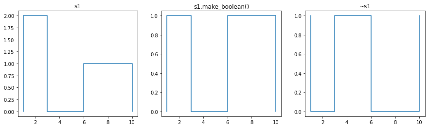
Lastly the ~ operator can be used to negate the make_boolean() result:

fig = plt.figure(figsize=(15, 4))

ax = fig.add_subplot(1,3,1)
ax.set_title("s1")
s1.plot(ax)

ax = fig.add_subplot(1,3,2)
ax.set_title("s1.make_boolean()")
s1.make_boolean().plot(ax)

ax = fig.add_subplot(1,3,3)
ax.set_title("~s1")
(~s1).plot(ax)

<AxesSubplot:title={'center':'~s1'}>